In the previous post, I had given a brief description of Linear Hashing technique. In this post, I will talk about Extendible Hashing.

Like Linear Hashing, Extendible Hashing is also a dynamic hashing scheme. First let’s talk a little bit about static and dynamic hashing as I had skipped this part in my previous post.

1. Static Hashing v/s Dynamic Hashing

Static Hashing uses a single hash function, and this hash function is fixed and computes destination bucket for a given key using the fixed number of locations/buckets in the hash table. This does not mean that the hash table that uses static hashing can’t be reorganized. It can still be reorganized by adding more number of buckets to the hash table. This would require:

• A new hash function that embraces the new size of hash table.
• Redistribution of ALL records stored in the hash table. Each record has to be touched and passed to the hash function to determine the new location/bucket. It is still possible that a record remains in the same bucket as it was before reorganization. But, hash function computation is definitely required for all the items in the hash table.

Dynamic Hashing tends to solve such problems:

• It gives the ability to design a hash function that is automatically changed underneath when the hash table is resized.
• Secondly, there is no need to recalculate the new bucket address for all the records in the hash table. For example, as explained in Linear Hashing, we split an existing bucket B, create a new bucket B*, and redistribute B’s contents between B and B*.
• This implies that rehash or redistribution is limited only to the particular bucket that is being split. There is absolutely no need to touch items in all the other buckets in the hash table.

Readers who have read the post on Linear Hashing should already be familiar with this dynamic hashing scheme. At this point, I would like to request the reader to first go through the post on Linear Hashing, as I personally consider it to be a bit simpler than Extendible Hashing.

Reading the post on Linear Hashing would lay a give a good background on dynamic hashing and prepare the reader for small complexities that will be talked about in Extendible Hashing algorithm. Moreover I refer to linear hashing technique in some parts of the post just to highlight the difference and also the uniqueness of both the approaches. So its better to read it first.

Now let’s talk about Extendible Hashing which is also another popular Dynamic Hashing method.

2. Extendible Hashing

Extendible Hashing is similar to Linear Hashing in some ways:

• Both are dynamic hashing schemes that allow graceful reorganization of the hash table, and automatically accommodate this fact in the underlying hash functions.
  • By “graceful”, I mean the luxury of not having to recompute the new location of all the elements in the hash table when the tale is resized. Redistribution or Rehash is limited to a single bucket.
• Both the schemes have a concept of bucket split. A target bucket B will be split into B and B* (aka split image of B), and the contents of B will be rehashed between B and B*.
• Hash Function used in both the schemes gives out a hash value (aka binary string), and certain number of bits are used to determine the index of destination bucket for a given key (and its value).
• The number of bits “I” used from the hash value is gradually increased as and when the hash table is resized, and more bucket(s) are added to the hash table.
• I would regard the last two points above as the fundamental principles behind these two dynamic hashing schemes.

However there are subtle differences between these two schemes when it comes to achieving a dynamic hashing behavior:

• Linear Hashing tolerates overflow buckets (aka blocks or pages). In other words, it is fine to have an overflow bucket chain for any given bucket in the hash table.
  • Extendible Hashing does not tolerate overflow buckets.
• In Linear Hashing, buckets are split in linear order starting from bucket 0 to bucket n-1, and that completes a single round of linear hashing. The bucket that is split is not necessarily the bucket that overflowed.
  • In Extendible Hashing, the bucket that is split is always the one that is about to overflow. This can be any random bucket in the hash table, and there is no given order on splitting the buckets.
• In Linear Hashing, there is just the hash table array comprising of buckets and per bucket overflow chain (if any). There is no auxiliary structure or any extra level of indirection.
  • In Extendible Hashing, an auxiliary data structure called as bucket directory plays a fundamental role in establishing the overall technique and algorithm. Each entry in the directory has a pointer to the main buckets in the hash table array. This gives an extra level of indirection. Before accessing the bucket, we first need to index the corresponding directory entry that has a pointer to desired bucket.
  • Just hold on to learn why a directory like structure is required in extendible hashing.

Bucket Directory

There are couple of strong reasons for using a bucket directory structure in extendible hashing.

• As mentioned earlier, there is no concept of overflow bucket chain in extendible hashing. This implies that when a given bucket B is full, we can’t resort to creating an overflow bucket and linking it to the chain of B as we did in linear hashing. The only thing that is possible is to split B, create a new bucket B*, and rehash contents of B between B and B*. After a split happens, the obvious question is how does the hash function correctly lookup the items that were earlier stored in B, but now in B* as a result of split ?
  • In Linear Hashing, the split was done in order. So if the split pointer S has moved ahead of the concerned bucket given by first hash function H, we know that this bucket was split. Thus we used the second hash function H1 to calculate the correct bucket (B or B*).
  • Readers who have gone through the post on Linear Hashing should be able to understand that the use of second hash function is equivalent to using one more bit from the hash value to get the correct bucket index.
  • We have to answer the same question for Extendible Hashing as well. The problem is that there is no such thing as a split pointer S, and the buckets are not split in linear order. Given any random bucket B that is about to overflow, we split it into B and B*. How do we know that we have to use 1 more bit from the hash value to index the correct bucket ?
  • Can we think of an auxiliary structure that embraces the fact that bucket was split, and points us to the correct bucket always ? This is where bucket directory structure comes into place.
• Bucket split is very crucial in extendible hashing. In linear hashing when an insert() detects a full bucket, it is anyways going to complete the operation by creating an overflow bucket and linking. Subsequently it will see if the condition for split is met or not. If yes, then the bucket pointed to by S will be split.
  • In extendible hashing when an insert() detects a full bucket, there is no way we can complete the insert at that moment because overflow chains are _NOT_ allowed. So the immediate action is to split, and then only the new item can be inserted somewhere.

Let’s discuss the data structure in more detail along with some examples.

Global Depth and Local Depth

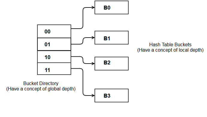
The above diagram shows the data structures for extendible hashing. There is a bucket directory, and the hash table buckets that store the records. Both the structure can be imagined in the form of arrays. Each location in the directory array has a pointer to some bucket.

Please do not make any assumptions about the relation between number of pointers from the directory, and the number of buckets in hash table. The diagram shows a simple 1-1 mapping, but this may not be true always. This will become clear as you read along.

The diagram clearly shows that any operation get(), put(), delete() on the hash table has to go through an extra level of indirection which is indexing the directory structure first and retrieving the bucket info.

Given a key K and hash function H, H has to map the key to a directory entry. This is where the global depth is used. Global Depth is equal to the number of bits used from the hash value generated by H. Let’s go with the “I” LSBs format as explained in linear hashing. So the integer value formed by “I” LSBs of the hash value is known as global depth and determines the index into directory structure.

Number of directory entries = 2^I. If 2 bits are used, we have 4 directory entries — 00, 01, 10, 11 as shown in the diagram.

On the other hand, local depth for bucket B is equal to “J” LSBs used from the hash value. The integer value formed by “J” LSBs of the hash value for key K really tells the actual number of bits used by the keys stored in bucket B. The following invariant always holds.

J (local depth) <= I (global depth)

Examples and Algorithms

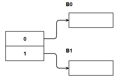
Start with 2 directory pointers and 2 hash table buckets. This tells that I=1 and also J=0 since the buckets are empty at the beginning. There is actually no harm in starting with J=I. Each bucket can store only 2 KV items.

Initial State:

Following put() operations are executed.

• put(4, V)
• put(1, V)
• put(7, V)
• put(2, V)

The steps are:

• Do the hash computation H(key) to get the bit string R.
• Use “I” LSBs from R as the directory index D.
• In our case the keys are simple integers, so H(k) = k is fine and R is just the binary representation of integer key K. However if K is a alpha-numeric value or anything other than plain integers, then H() has to do some computation to throw out R and this is typical for any hash function.
• All we need is to get the value of “I” LSBs from R and this will give us D.
• Go to the directory location D, follow the bucket pointer to get the desired bucket B.
• Store the item in bucket B.

For any given bit string R, if we want “I” LSBs from the binary representation of the number, the best way to do is N%(2^I). This perfectly works here because the directory structure we are trying to index is always in powers of 2 — 2, 4, 8, 16 etc. This is something also used in Linear Hashing.

• H(4) = 4 = 0100 ; I => 4%2 = 0 ; 0100 (the LSB is highlighted).
• H(1) = 1 = 0001 ; I => 1%2 = 1 ; 0001
• H(7) = 7 = 0111 ; I => 7%2 = 1 ; 0111 
• H(2) = 2 = 0010 ; I => 4%2 = 0 ; 0100

Note that as long as the bucket has space to store the item, we do not need any sort of fancy stuff like splitting etc.

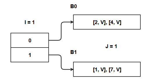
At this time, our hash table is full. J = I = 1. J started out as 0, and was set to the value of I upon first insert in an empty bucket.

We then do put(22,V)

H(22) = 22, and D = 22%2 = 0 = 00010110 which points to B0. The target bucket is already full, and we can’t create an overflow chain. We split B0 as follows:

• Split of B0 to [B0, B0*] will create an additional hash table bucket. Two things are required:
  • To be able to track the new bucket through directory.
  • To be able to correctly locate items after rehash between B0 and B0*.
• We do not have additional space in the directory. With 1 bit we can only have 2 directory index locations. So we need more than 1 bit which comes by incrementing global depth by 1.
• This causes the directory to double, and give us the following directory locations:
  • 00, 01, 10, 11 because now we are using 2 bits from hash value (I = 2).
• Create bucket B0* as the split image of B0.
• Increase the local depth J of B0 by 1, and set this as the local depth of B0* as well. Why is this step required ?
  • It is because the bucket is being split. We will now use 1 more bit to pick up the destination directory and bucket for the items.
  • Items stored in B0 and B0* will no longer be stored using the only LSB. 2 LSBs will be be used henceforth.
• Store a pointer in one of the new directory locations to bucket B0*. How do we determine which directory location D ? Because we are using 1 more bit from the hash value, D0 which was pointing to B0 should now have a companion D* location that points to B0*. How do we get D* ?
  • It simple !!. We have added 1 more bit to I, so D0 and D* should point to buckets B0 and B0* that have the LSB common since earlier I was 1.
  • So D* = D0 + 2^(old global depth) = 0 + 2^1 = 2 =  bucket directory 10.
• Note that directory pointer to bucket that is split remains unchanged.
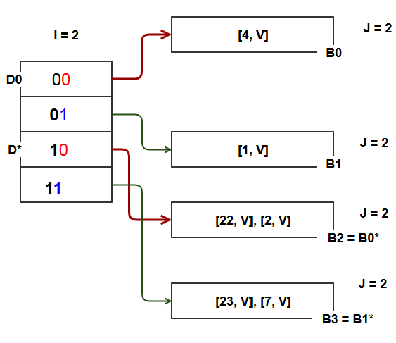
• Execute Put(22, V) and do a rehash of keys 2 and 4 since they were earlier stored at B0 and may move to to B0*.
  • H(22) = 22 = 00010110 ; D = 22%(2^I) = 22%4 = 2. Hence directory 10
  • H(2) = 2 = 0000010 ; D = 2%(2^I) = 2%4 = 2. Hence directory 10
  • H(4) = 4 = 00000100 ; D = 4%(2^I) = 4%4 = 0. Hence directory 00.

The highlighted red/violet bits in the directory location suggests that items stored in the bucket pointed to by these respective directories share the LSB but not both LSBs.

For example items stored in B0 and B0* share the LSB as 0. Items store in B0 share both the LSBs as 00. Items stored in B0* share both the LSBs as 10.

In the diagram we see bucket B1 is being pointed to by directories 01 and 11.It was already pointed to by 01 earlier, then why is there a need to create a pointer from new directory location 11 ?

Also why was the local depth of B1 not incremented ?

• The reason is that bucket directory has now doubled in size. “I ” will be used as 2 in all the subsequent hash computations for put(), get(), delete() operations.
• The items 1 and 7 stored in B1 were stored using I as 1. Now that I is 2, they may or may not have both the LSBs in common.
• B1 has to stay the same as it is not split. So all the items currently in B1 will remain in B1. Hence local depth can’t be increased as keys 1 and 7 are stored in their destination bucket B1 using I as 1.
• Since any get() will now use the 2 LSBs, there is a chance that the 2 LSBs for these keys are “11”, and because there is no pointer from directory 11, reader will miss out the entry.
• In the current case, this will happen for key 7 (0111) where D = directory 11.Hence there is a need to store the pointer. This will become more obvious with the next split example.

Put(23, V) ; 23 = 00010111 D = 23%4 = 3 = directory 11. This points to B1 which is full. We will have to split it.

• This time we don’t need to double the size of directory as we did during earlier split.
• The directory is already prepared to accommodate the split since split of B1 means using 2 LSBs instead of 1. The directory is already using 2 LSBs and has 4 locations.
• Create split image of B1 as B1*. Items in B and also the new item 23 will go either to B1 or B1* depending on whether there 2 LSBs are 01 or 11.
• Global depth I remains the same since directory size is not changed. Local depth J of B1 and B1* is incremented by 1 since keys stored in these buckets will be using 1 more bit from the hash value.

 

Put(18, V) ; H(18) = 18 = 00010010 , D = 18%4 = 2 => directory 10 that points to bucket B2. B2 is full, and we will split B2.

• Current global depth is 2 and local depth at B2 is also 2. So when B2 splits and we start using 3 bits from the hash value, we can’t really do that without doubling the directory size from 4 to 8 and thus incrementing I to 3.
• A new split image of B2 is created as B2*. Pointers in directory locations are stored as explained before. Note the multiple pointers to buckets B0, B1, and B3. These buckets aren’t yet split and still at local depth of 2. But because directory has doubled and I has gone up by 1 bit, we need these additional pointers.

The fundamental concepts behind put() are:

• If the target bucket B has space, store the items there. Simple and sweet !!
• If the target bucket B is full:
  • If the local depth J of B is less than global depth I, then split the bucket but there is no need to double the directory as the directory is already prepared for the split (as J < I). This is actually the case of multiple pointers to a single bucket.
  • If the local depth J of B is equal to global depth I, then double the directory (equivalent to incrementing I), and split the bucket. Because J==I, there is no way for us to create a split and increment J without incrementing I. So the directory has to be doubled to accommodate the split.
  • In any case when the bucket B is split, its local depth J is always incremented by 1, and this will also be the local depth of split image B*.

So in the above diagram:

• If bucket B0, B1, B3 reach to a point of split, the directory size will still remain 8 as the local depth at these buckets is less than global depth.
• However if buckets B2 or B4 reach a split point, then it would require incrementing I since the local depth is already equal to global depth and the current state of directory will not be able to manage the split. The directory will be doubled to 16 locations and I will be 4.

In this post, and the previous post on Linear Hashing, I have only described how these approaches work, and explained some algorithms. In my subsequent posts, I will try to compare the two schemes and also give pointers to implementation along with some more interesting examples.